www.slide4math.com

This is my version of explanation. I would suggest you to come up with your own explanation. The best way would be for you to try explain this to somebody else in your own words.

Following is my version of explanation, but this is just an example. You may come up with a better version.

What is exponential function ?

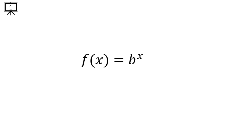
[Slide 1] Exponention Function is a function expressed as on this slide. The base (b) is a number (real or complex number) and the exponent (x) is the independent variable.

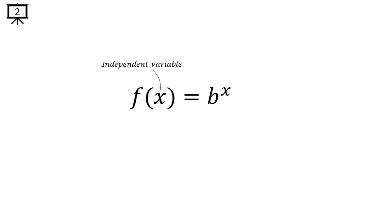
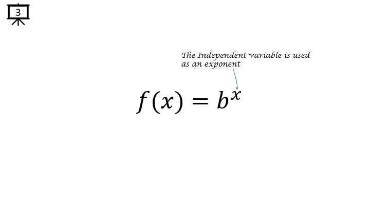
[Slide 2, 3] As shown on this slide, the variable x is the independent variable of the function.

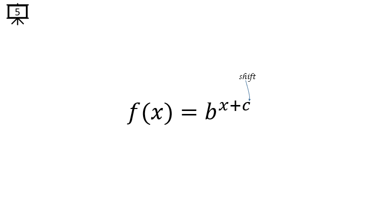
[Slide 5] As in any other function, you can shift the graph of a function by adding a constant to the independent variable.

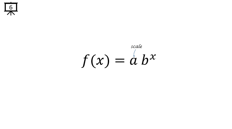
[Slide 6] You can scale the function by multiplying a constant (or another function) to the base function.

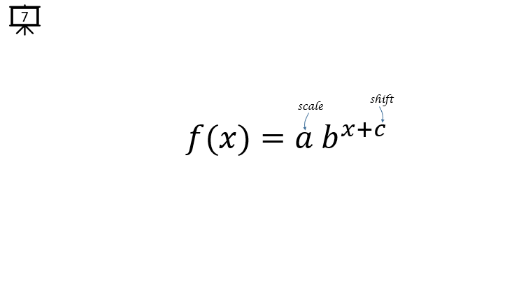
[Slide 7] With this form, you can both scale and shift the base exponential function.

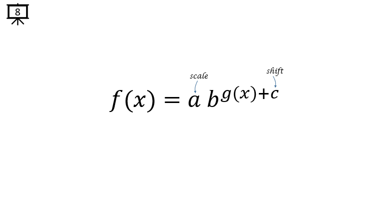
[Slide 8] In some case (actually in many application of exponential function), the exponent part of the function can be another function (g(x)) as on this slide (you will see many of this case in application pages for exponential function).

[Slide 9] From this slide, you will see some of basic examples of exponential functions in the form of graphs.

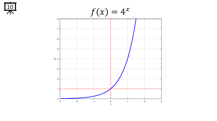
[Slide 10] This is an example of exponential function with the base of 4. In the whole range of x (independent variable : Horizontal axis), the y value increases as x increases. When x is negative value, y increases slowly between 0 and 1. At x = 0, the y value becomes 1. When x is positive value, y value gets drastically.

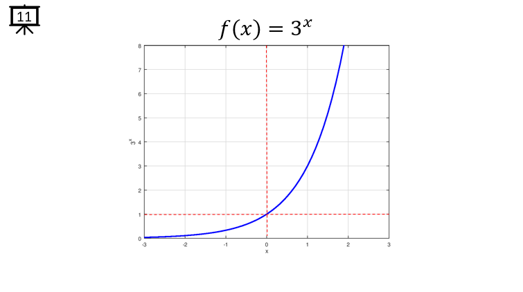
[Slide 11] This is an example of exponential function with the base of 3. The overall tendancy of the graph is same as in [Slide 10].

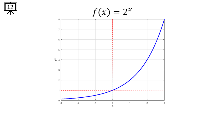
[Slide 12] This is an example of exponential function with the base of 2. The overall tendancy of the graph is same as in [Slide 10] as well.

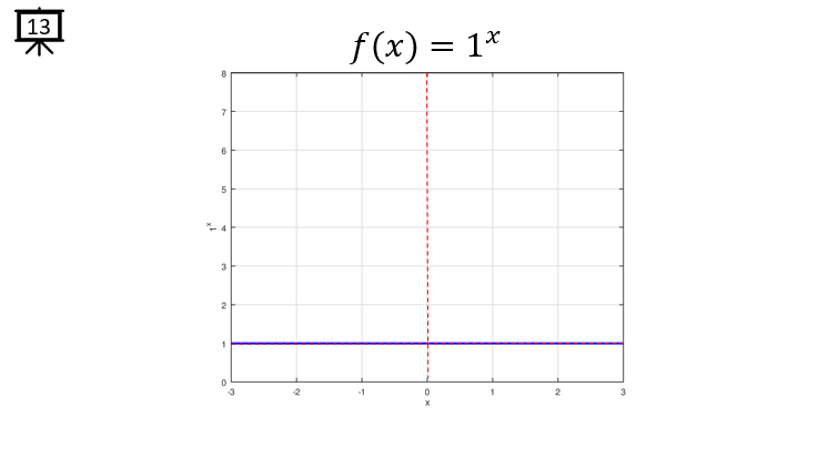
[Slide 13]  This is an example of exponential function with the base of 1. Now you would see the differences from previous example. On this graph, you see the y value stays same (i.e, the value of 1) regardless of the exponent x value.

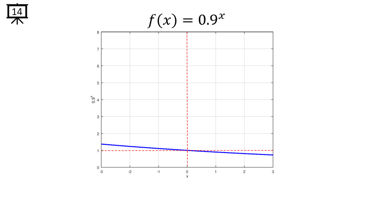
[Slide 14]  This is an example of exponential function with the base of 0.9. This is an example of the base being less than 1. In this graph, the overall graph decrease as x value increases. When the x value is negative value, the y value declines above 1 and reaches to the number 1 when x is 0 and then contines to decrease below 1 when x is positive value.

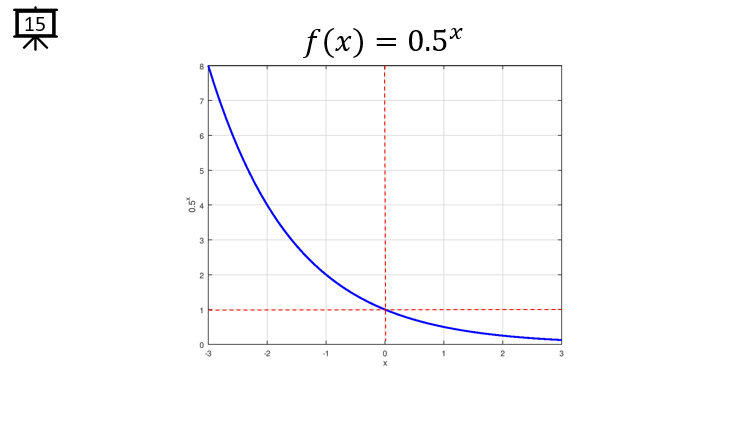
[Slide 15]  This is an example of exponential function with the base of 0.5. The overal trend is similar to [Slide 14], the difference is that the slope of decrease gets larger comparing to [Slide 14].

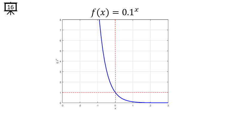
[Slide 16]  This is an example of exponential function with the base of 0.1. The overal trend is similar to [Slide 15], the difference is that the slope of decrease gets larger comparing to [Slide 15].

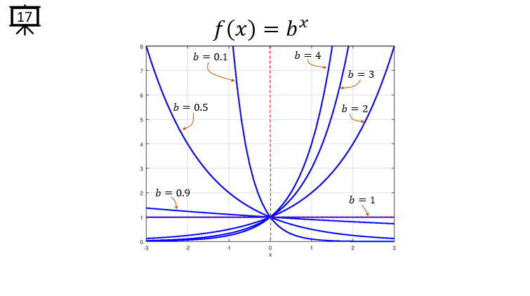
[Slide 17] Now I put all the plots of the examples onto a single graph. Can you try to notice how each of the plot changes depending on the base values ? I don't think I need to put any additional comments here. Only a comments I want to point out is that the y value at x = 0 is all same ( y = 1) regardless of the base value of the exponential function.

< Code 1 >

: Following is the Octave code that I wrote to plot the graphs in this page.

x = -3:0.1:3;

a = 1;

y = b .^ x;

plot(x,y,'b-','Linewidth',2);

ylim([0 8]);

set(gca,'ytick',0:1:8);

grid on;

< Code 2 >

: Following is the code for the plot showing the multiple graphs in a single plot. You may change the values (or number of values) in aList and try.

x = -3:0.1:3;

bList = [4 3 2 1 0.9 0.5 0.1];

hold on;

for b = bList

y = b .^ x;

plot(x,y,'b-','Linewidth',2);

ylim([0 8]);

end

hold off;

set(gca,'ytick',0:1:8);

grid on;